Blog: Middle Temperature Error
Date: 2 February 2017
Copyright © David Boettcher 2005 - 2026 all rights reserved.I make additions and corrections to this web site frequently, but because they are buried somewhere on one of the pages the changes are not very noticeable, so I decided to create this blog section to highlight new material. Here below you will find part of one of the pages that I have recently either changed or added to significantly.
The section reproduced here is from my page about Temperature Effects in Watches.
If you have any comments or questions, please don't hesitate to contact me via my Contact Me page.
Middle Temperature Error
HSN article about Middle Temperature Error.
Download article: MTE.pdf A5771
Download spreadsheet: MTE.xlsx S4082 I4026
In the late eighteenth century a phenomenon was observed in marine chronometers with temperature compensation. It was found that if the device was brought to time at a certain temperature it would lose at higher and lower temperatures. This effect was not observed in watches without temperature compensation because it was dwarfed by other effects, principally the change in rate with temperature due to variation in the elasticity of the balance spring. The effect became observable in marine chronometers with compensation for this major, primary source, of temperature caused error.
To minimise the total error over the range of temperatures a marine chronometer was expected to encounter, the timing was adjusted so that it was fast at a "middle" temperature and correct at two temperatures either side of this. This gaining rate at the middle temperature was called the "middle temperature error". Because the effect only became noticeable once the primary source of error, the change in the elasticity of the balance spring with temperature, had been compensated, it was also sometimes called "secondary error".
The cause of middle temperature error has been much debated over the years since it was first observed. Qualitative explanations were advanced claiming that it was due to the effects of square or square root terms in the equation for the period of a balance. Although these explanations were logical and true, it has now been shown quantitatively that the magnitude of the error they cause is much smaller than the errors observed in practice. This is briefly outlined further down on this page and if you are not already familiar with recent discussions around middle temperature error I suggest that you read that short summary first.
This is discussed in more detail in an article published in the February 2017 edition of the Horological Science Newsletter (HSN). The article introduces a spreadsheet model that demonstrates the magnitudes of the different effects that contribute to middle temperature error. The HSN newsletter is published by NAWCC Chapter #161. The interest of Chapter #161 is the study and distribution of information about the science of horology. Chapter membership is available to members of the NAWCC. The editor of HSN, Bob Holmström, kindly agreed that my article and accompanying spreadsheet can also be downloaded from this web page.
The spreadsheet that accompanies the article allows you to interactively explore the effects of temperature on a balance and balance spring. I strongly recommend that you download and try it. You don't need to do any spreadsheet programming, it is already set up. You just alter the values of the thermal coefficients of expansion and elasticity, and charts built into the spreadsheet immediately show you the effect on timekeeping. It's really simple so give it a go, and if you have any problems just drop me an email. The spreadsheet is in Excel format. If you don't have the Microsoft Office Excel spreadsheet software, then Libre Office contains an excellent alternative that can open Excel format spreadsheets and is available absolutely free from Download Libre Office.
Spreadsheets were created to simplify and automate business models originally created with chalk and blackboards. They are a powerful tool, easy to use and incredibly useful but, like all complicated tools, if you have never been shown how to use one they can be initially daunting. I have created a very short and quick introduction into how they work to get you going. Download it from this link: Spreadsheets – A Quick Introduction (pdf). NB: Updated to Rev. 2.0 on 28 November 2017.
The spreadsheet can also be used to investigate the effects of the individual components. For example, to see the effect of thermal expansion of the balance alone, then set all the coefficients apart from the "Thermal expansion/ºC – balance:" to zero. As a check, a brass balance should show a loss of 1.64 seconds per day for a temperature increase of one degree C, a steel balance 0.95 seconds per day per degree C. The loss occurs because thermal expansion of the balance increases its rotational inertia, the difference in rates is because of the smaller thermal expansion of steel than brass.
The article and spreadsheet can be downloaded from these links: Article: MTE.pdf, Spreadsheet: MTE.xlsx.
If you have any comments or questions, please don't hesitate to contact me via my Contact Me page.
Explanations of Middle Temperature Error
An explanation for middle temperature error was developed by the Reverend George Fisher and published in The Nautical Magazine of 1842 under the name of E. J. Dent, of the chronometer makers Arnold & Dent. Fisher's name is not mentioned in Dent's article, most likely because Fisher had incurred the displeasure of the English chronometer industry by publishing a paper that suggested that the going of chronometers could be affected by magnetism in iron ships, which was wrong but potentially damaging to the chronometer industry, and Fisher probably decided to keep a low profile as a result. He continued to work on chronometers but didn't publish anything further about them.
The explanation published by Dent was based on the observation that the equation for the period of a balance controlled timepiece can be written as:
$$ T = {2 \pi} \sqrt \frac { m k^2}{S} $$where mk2 is the moment of inertia of the balance, m being the mass and k the radius of gyration, and S represents the force or turning moment exerted by the balance spring.
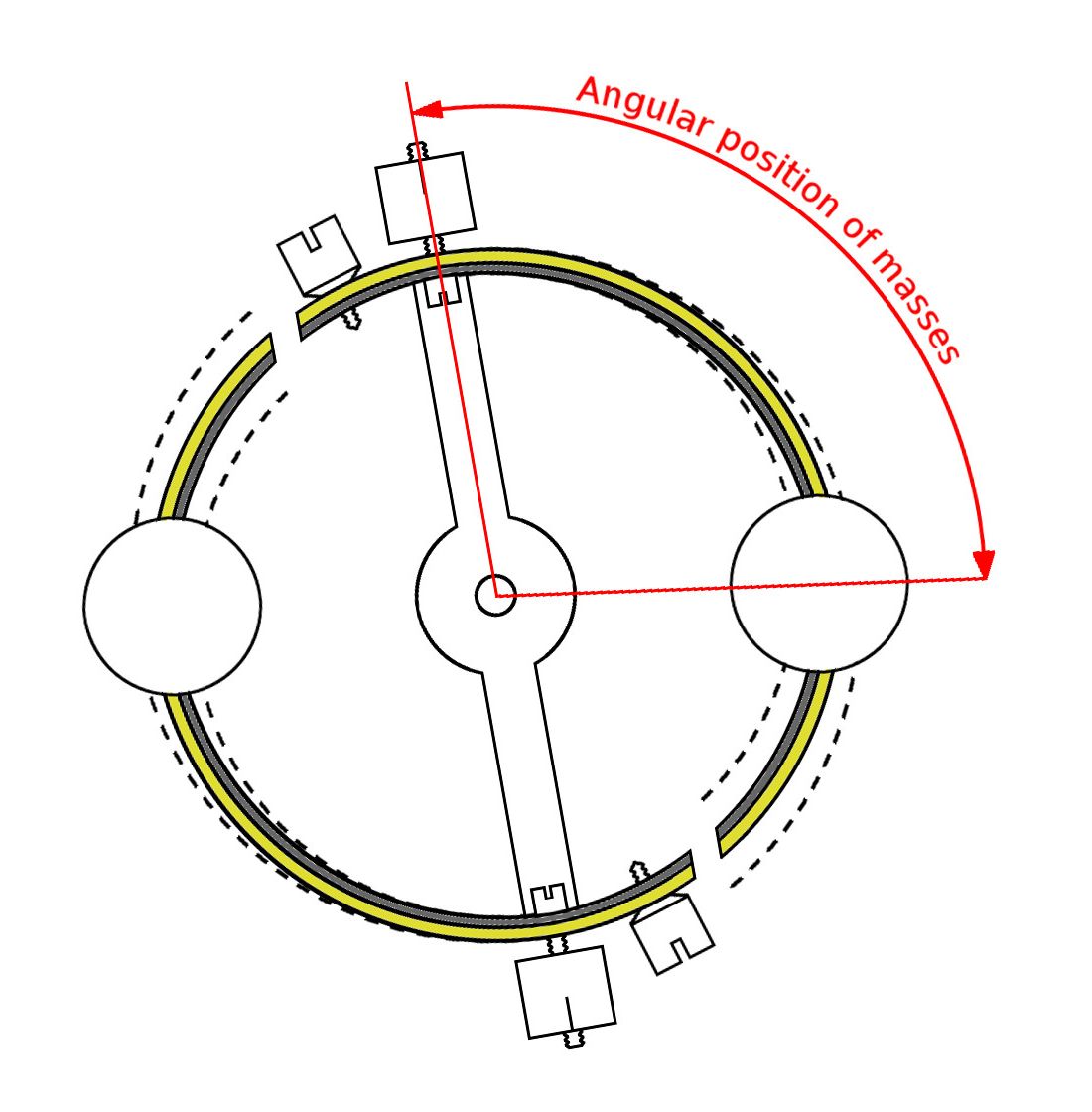
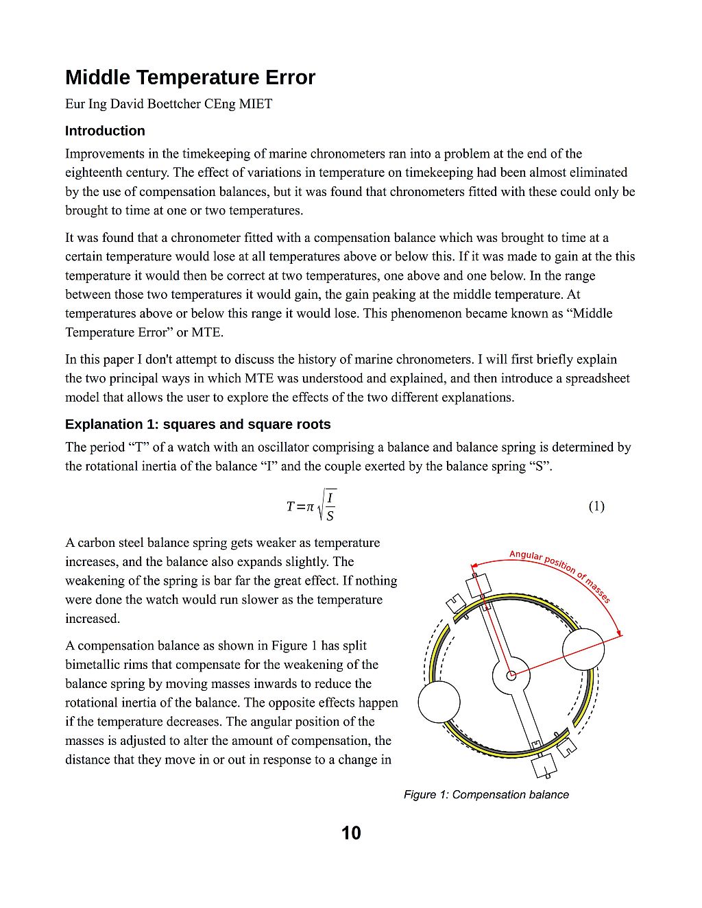
Marine chronometer compensation balance
A bimetallic compensation balance alters the radius of gyration k in response to changes in temperature. The balance shown in the image illustrates how this happens. The rim of the balance is made by fusing brass onto the outside of a steel balance, and then making two cuts through the rim near to the spoke. If the temperature increases the brass expands more than the steel, which causes the bimetallic secions to curve inwards. If the temperature falls, the brass contracts more than the steel which makes the bimetallic secions curve outwards. The bimetallic secions carry masses and the radial position of these masses alters the moment of inertia of the balance. The amount of compensation can be altered by sliding the masses along the bimetallic secions. The further along the bimetallic secions that they are positioned, the greater the compensation.
If the temperature increases, the elastic force exerted by the balance spring decreases and the bimetallic sections of the balance move the compensation masses inwards to reduce the rotational inertia. The opposite happens for a fall in temperature, the bimetallic secions move the compensation masses outwards. The masses move only a very small distance and it seemed likely that they moved proportionally in response to temperature changes. Observations by Dent had suggested that the elasticity of the balance spring varied linearly with temperature, or very nearly so. In fact, Dent's data does show a non-linear effect in the spring tension, but for the purposes of explanation he assumed that it was negligible.
If the compensation was to be perfect, then from the equation above it is clear that the ratio of \(k^2\) to \(S\) must be constant. But if the masses are moved proportionally to a change in temperature, then the change in \(k\) will be linear and \(k^2\) will be a quadratic curve. Fisher realised that the curve produced by plotting \(k^2\) against temperature on a chart could only intersect with a straight line representing a linear \(S\) term at either one or, at most, two points. This is the explanation related by Commander Gould in "The Marine Chronometer" and drawn in a figure as a series of "I" curves representing the moment of inertia against a straight "S" line representing the spring term.
The Fisher / Dent explanation considers the relationship of the balance's moment of inertia to spring force within the encompassing square root sign of the equation for period. However, the encompassing square root cannot be ignored. When it is taken into account, it is evident that the period is proportional to the square root of \(k^2\); that is, the period is directly proportional to \(k\). It is clear from this that whatever is the source of the non-linearity that gives rise to middle temperature error, it is not the square in the inertia term.
An alternative way of visualising the effect is to rewrite the equation for period as:
$$ T \propto \frac { k} {\sqrt S} $$If both k and S vary linearly with temperature, as was supposed, then a plot of k against temperature on a chart would be a straight line, but the plot of S would be a quadratic curve due to the square root. The k line could only intersect with the curve of the S term at either one or, at most, two points. This is the explanation related by A. L. Rawlings in "The Science of Clocks and Watches".
The “square root” explanation is rational, logical and correct, and it held sway as the only explanation for middle temperature error for many years. However, although the reasoning is correct, the magnitude of the middle temperature error produced by this effect is much smaller than that actually observed. There must be another, more significant, factor at work.
The shortcoming in the square root explanation was noticed by Peter Baxandall during the updating of Rawlings' classic work by the BHI, and subsequently investigated by Philip Woodward in a paper published in the Horological Journal of April 2011. Woodward showed that the middle temperature error produced by the square root effect alone was around one tenth of a second per day, only a small fraction of observed values.
The reason that the square root effect is so small is because all of the coefficients are close to unity, where unexpected things happen to square roots. Lets say we are interested in a temperature range of 30°C; that's +/- 15°C around the middle temperature. The variation in the elastic modulus is given by 1+αt, where α (alpha) is the thermoelastic coefficient and t is the temperature change. Using Rawlings' figure of -207 parts per million per °C for the thermoelastic coefficient for S (he calls it Q), at the extremes of temperature +/- 15°C the change in the stiffness of a balance spring will be 0.9969 at +15°C and 1.0031 at -15°C.
Let's just look at the second of these figures for a moment. We want the square root of 1.0031 to use on the bottom of the equation for period. Rather than reaching for a calculator, lets look at the Taylor series expansion:
\[ \sqrt{1+x} = 1 + \frac{x}{2} - \frac{x^2}{8} + \frac{x^3}{16} ... \]Here the value of 1.0031 can be substituted for 1+x, with x = 0.0031. The third term in the series, x squared over two, will be very small and it, along with all subsequent terms, can be neglected. So when x is small like in this case, the square root of 1-x can, with a high degree of accuracy, be represented by:
\[ \sqrt{1+x} = 1 + \frac{x}{2} \]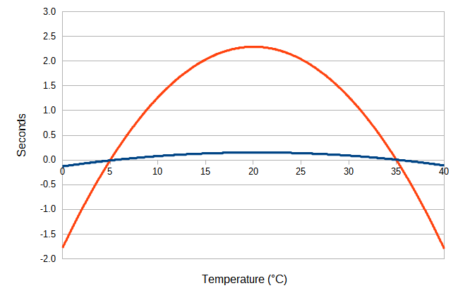
Middle temperature error or secondary error: seconds per day.
1: Blue line; square root effect alone.
2: Orange line; square root plus non-linear elasticity of balance spring.
It is immediately apparent that if the square root of the thermoelastic changes between +/- 15°C can be represented to a high degree of accuracy by the linear term on the right of the equals sign, the relationship between temperature and the stiffness of the spring is, also to a high degree of accuracy, linear. There is no doubt that the square root does cause some non-linear effect, but it is tiny. A cause for vast bulk of the middle temperature error must be sought in a different explanation.
The chart here shows the two effects on the timekeeping of a machine brought to time at 5°C and 35°C, with a middle temperature of 20°C. The blue line shows the middle temperature error that results from the square root explanation alone. It is very small, of the order of one tenth of a second per day. The orange line shows the error that results when the curvature in the temperature response of the elasticity of the balance spring is also taken into account. This results in an error of more than two seconds per day, which is in accordance with observed values of middle temperature error.
The Cause of Middle Temperature Error
In the late nineteenth century, Dr Guillaume noted that middle temperature error, which he called ‘secondary error’ or ‘Dent’s error’, is significantly reduced when a palladium alloy balance spring is used instead of a steel one. Palladium springs require slightly more overall temperature compensation than steel springs, so the reduced error is not due to smaller changes in the modulus of elasticity with temperature. It occurs because the modulus of elasticity in palladium alloys varies more linearly across the temperature range than that of steel.
The non-linear behaviour of steel springs is primarily due to their magnetic properties and crystal structure. Steel is ferromagnetic at room temperature, and changes in magnetic domain structure contribute significantly to non-linear variations in elasticity as temperature changes. Modern studies on magnetoelasticity confirm that these magnetic effects are a major source of non-linearity in the temperature–elasticity relationship for steel.
By contrast, the palladium alloys used for balance springs are non-magnetic, eliminating a major source of non-linear behaviour. In addition, palladium alloys typically have a face-centred cubic (FCC) crystal structure, which provides a more symmetrical and stable atomic arrangement than the body-centred tetragonal (BCT) or martensitic structures found in many spring steels. As a result, palladium alloy springs exhibit a more linear change in modulus of elasticity with temperature. Other effects, such as thermal expansion and alloying, play a role but have much smaller influence in comparison.
It is not clear that Guillaume ascribed any of the middle temperature error to the square root effect, he doesn't mention it in his writings. Dr Guillaume's solution to the problem of the middle temperature error can be found at The Guillaume "integral" balance.
Further Reading
There is more about temperature effects in watches, compensation balances, and special metals that were developed for the balance spring, on my page about Temperature Effects in Watches.
If you have any comments or questions, please don't hesitate to get in touch via my Contact Me page.
Copyright © David Boettcher 2005 - 2026 all rights reserved. This page updated December 2025.
Back to the top of the page.